Advanced PostgreSQL Partitioning by Date with YugabyteDB Auto Sharding

Recently, I wrote about how YugabyteDB can scale without having to use PostgreSQL declarative partitioning and working around its limitations. I referenced a table from Kyle Hailey’s blog detailing a PostgreSQL production issue involving a “payments” table, where “payment_id” is the primary key. Kyle’s post pointed out that including a partition key in the primary key is mandatory in PostgreSQL.

In my blog post, I discussed the scaling process and explained how to hash shard the “payments” table on the “payment_id” without changing its primary key. This method ensures fast inserts by distributing the table rows across the cluster’s nodes. This approach works seamlessly with YugabyteDB’s automatic sharding and supports the use of any secondary index for additional use cases.

I received some feedback on Reddit and other sites that partitioning on a different column may be better. This is true for PostgreSQL, where the partition key limits the partitioning of the table and all the indexes. However, with YugabyteDB sharding, I don’t need to change the table partitioning to query a range of dates. YugabyteDB’s secondary indexes are global, meaning they don’t need to share a sharding key with their table. In addition, distributing the rows in a distributed PostgreSQL database like YugabyteDB offers extra benefits since it spreads data across multiple active servers.

To query a range of dates, you can create an index on the date and add more columns for an Index Only Scan. When defined as ascending or descending, this index will be range-sharded and distributed based on its key. Here’s an example:

create index on payments ( created ASC, payment_id ) include ( amount );

If you have a reason to partition the table by date to group close dates together, you can also do that in YugabyteDB. Here is an example.

Sharding by a Range of Dates

I’ve modified the table’s primary key to include the “created” column, similar to how you would partition in PostgreSQL.

create table payments (
       primary key (created ASC, payment_id)
     , unique(payment_id)
     , payment_id bigint not null generated always as identity (cache 1000)
     , created timestamptz not null default now()
     , account_id bigint not null
     , amount decimal(10,2) not null
)
split at values ( ('2001-01-01'),('2002-01-01'),('2003-01-01'),('2004-01-01') )
;

My reasoning behind this approach includes three key points.

1. I set payment_id as a unique key to ensure it’s indexed and enforced with no duplicates. In SQL, a unique key with non-nullable columns is similar to a primary key. The main difference is its physical organization. By starting the primary key with the “created” date, I can group close dates together, which is useful when date range queries are the critical access pattern vs. distributing the inserts.
2. I added ‘ASC‘ to the primary key because YugabyteDB defaults to ‘HASH‘ on the first column of the primary key. Since I want to organize the table by a range of dates, I do not want to apply a hash function to this column. If you frequently query for the latest date with ‘order by created desc limit 10‘, then it is better to avoid a backward scan and define it as ‘DESC‘. Both options allow for range sharding.
3. Although not mandatory (because the table will be split automatically by YugabyteDB as it grows), I added ‘split at values‘ clause to pre-split the table to five tablets. In my previous blog, I demonstrated that the number of tablets could number in the hundreds or thousands. While it is possible to pre-create hundreds of tablets by providing more splitting values, I opted for simplicity and stuck to the auto-splitting thresholds.

The table is empty with five tablets, and the hash-sharded index for the unique constraints has one tablet per node:

yugabyte=> select num_tablets from yb_table_properties('payments'::regclass);
 num_tablets
-------------
           5
(1 row)

yugabyte=> select num_tablets from yb_table_properties('payments_payment_id_key'::regclass);
 num_tablets
-------------
           9
(1 row)

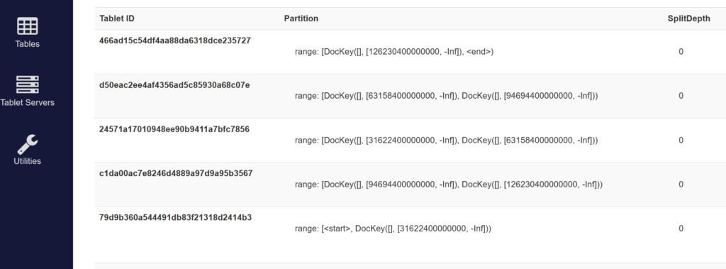
I can view the tablet boundaries from the console, which shows the data ranges in their internal int64 representation, which0 corresponds to the PostgreSQL Epoch (number of microseconds since Jan 1st, 2000):

Auto-Splitting: Let’s Insert a Hundred Million Rows

I will insert the same number of rows as I did in the previous blog: a hundred million.

yugabyte=> insert into payments (account_id, amount, created)
 select 1000 * random() as account, random() as amount,
 random() * interval '24.25 year' + timestamp '2000-01-01 00:00:00' as created
 from generate_series(1,100000) account_id
\watch c=1000

While the table was growing, the tablets were split, and more tablets became visible in the console. “SplitDepth” counted the number of automatic splits that resulted in each tablet.

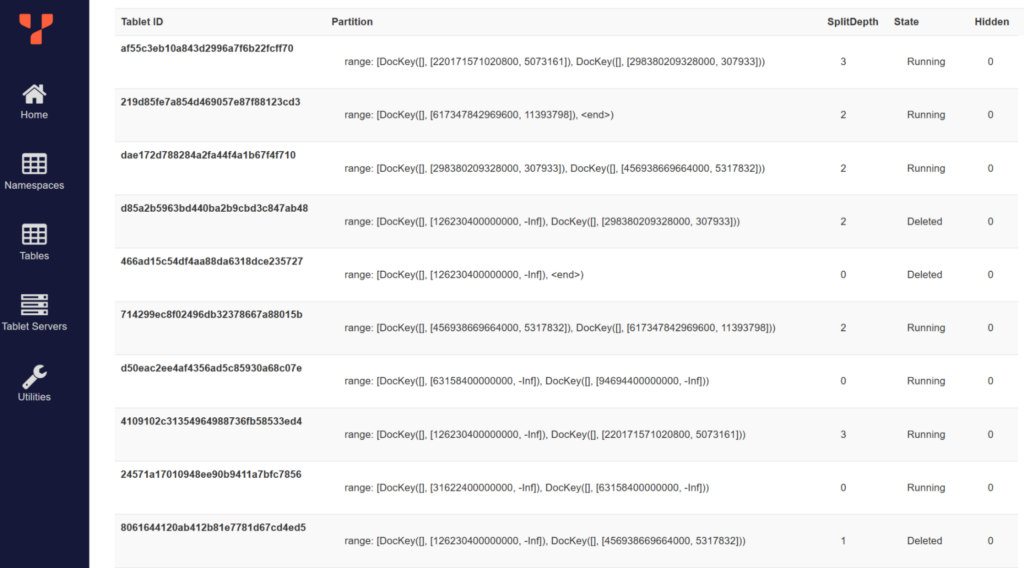
At the end of the load, I have 17 tablets for the table (ranges of date) and the same for the unique index (by hash).

yugabyte=> select num_tablets, pg_size_pretty(pg_table_size('payments')) from yb_table_properties('payments'::regclass);

 num_tablets | pg_size_pretty
-------------+----------------
          17 | 5738 MB
(1 row)

yugabyte=> select num_tablets, pg_size_pretty(pg_table_size('payments_payment_id_key')) from yb_table_properties('payments_payment_id_key'::regclass);

 num_tablets | pg_size_pretty
-------------+----------------
          17 | 4527 MB
(1 row)

yugabyte=>

To view the number of tablets created by range sharding, you can utilize the yb_get_range_split_clause() function. This function provides the range clause needed if you want to replicate the table with the same tablet division:

yugabyte=> select yb_get_range_split_clause('payments'::regclass);
                                                                                                                                                                                                                                                                                                                                        yb_get_range_split_clause                                                                                                                                                                                                                                                                                       
-----------------------------------------------------------------------------------------
 SPLIT AT VALUES (('2001-01-01 00:00:00+00', MINVALUE), ('2002-01-01 00:00:00+00', MINVALUE), ('2003-01-01 00:00:00+00', MINVALUE), ('2004-01-01 00:00:00+00', MINVALUE), ('2005-07-24 14:37:18.5088+00', 2040738), ('2006-12-29 17:30:45.9936+00', 13050457), ('2009-08-15 00:22:12.5472+00', 15029518), ('2010-12-14 10:55:54.6816+00', 46169115), ('2011-12-30 05:40:38.8704+00', 38646207), ('2014-04-03 01:05:37.4208+00', 5689338), ('2015-10-23 17:18:36.1728+00', 16944332), ('2017-04-06 17:42:07.8624+00', 14921933), ('2018-08-19 21:15:27.6768+00', 63227870), ('2019-10-15 04:40:06.528+00', 8756978), ('2021-02-02 10:10:58.3968+00', 37865384), ('2022-05-14 02:18:22.8672+00', 27792641))
(1 row)

yugabyte=>

From this, it’s clear that range sharding considers the entire key. Therefore if a huge amount of data is loaded for the same date, it can be split further within the same date.

Query on a Range of Dates: 80000 Rows in 250 Milliseconds

Remember, my primary goal when partitioning on the date was to query a range of dates.

yugabyte=> explain (analyze, dist, costs off, summary on)
          select * from payments
          where created between date '2023-12-25'::timestamptz
                            and '2024-01-02'::timestamptz
          order by created
;
                                                                   QUERY PLAN
------------------------------------------------------------------------------------
 Index Scan using payments_pkey on payments
 (actual time=3.568..246.471 rows=80142 loops=1)
   Index Cond: ((created >= ('2023-12-25'::date)::timestamp with time zone) AND
                (created <= '2024-01-02 00:00:00+00'::timestamp with time zone))
   Storage Table Read Requests: 79
   Storage Table Read Execution Time: 202.721 ms
 Planning Time: 0.065 ms
 Execution Time: 250.869 ms
 Storage Read Requests: 79
 Storage Read Execution Time: 202.721 ms
 Storage Execution Time: 202.721 ms
 Peak Memory Usage: 8 kB
(14 rows)

This approach splits data into date ranges to keep the table size manageable and keeps the rows sorted in the LSM Tree. As a result, it eliminates the need for an extra Sort operation for ORDER BY.

Query on a Global Unique Index in 2 milliseconds

The additional UNIQUE key on payment_id can be used to get fast access to the table’s business key because our primary key is now a surrogate key with a different order:

yugabyte=> explain (analyze, dist, costs off, summary off )
          select * from payments
          where payment_id = 42
          order by created
;
                                              QUERY PLAN
----------------------------------------------------------
 Sort (actual time=4.105..4.105 rows=1 loops=1)
   Sort Key: created
   Sort Method: quicksort  Memory: 25kB
   ->  Index Scan using payments_payment_id_key on payments
     (actual time=4.094..4.097 rows=1 loops=1)
         Index Cond: (payment_id = 42)
         Storage Table Read Requests: 1
         Storage Table Read Execution Time: 2.840 ms
         Storage Index Read Requests: 1
         Storage Index Read Execution Time: 1.080 ms
(9 rows)

Since the index being used is not the primary index, it is necessary to access the table to retrieve values for the other columns, leading to a Table Read Request and an Index Read Request. However, since it is a unique identifier queried by value and sharded by hash, it will read only one row. The additional “hop” to the table is limited to one read request per query. Despite sounding counter-intuitive, declaring the business key with a unique constraint and using the primary key for another purpose is the right way to go. This is because the business key can be overloaded with a clustering key to store together that which is often queried together.

Secondary Indexes for Additional Use Cases

In the previous blog, I created an index to access by “account_id”.

create index payments_by_account on payments(account_id, amount desc)
;

yugabyte=> select num_tablets, pg_size_pretty(pg_table_size('payments_by_account')) from yb_table_properties('payments_by_account'::regclass);

 num_tablets | pg_size_pretty
-------------+----------------
           9 | 3513 MB
(1 row)

Creating more secondary indexes does introduce overhead during insertions, deletions, or updates of the columns in the index. However, this overhead is minimal in YugabyteDB compared to traditional databases. Databases that use B-Tree, like Oracle, PostgreSQL, or SQL Server, require multiple reads and writes to insert a new index entry—finding the leaf block from root to branches, updating it, and (when full) splitting it and updating the branches. YugabyteDB’s LSM-Tree structure allows fast index entry inserts by appending the new entry directly to the MemTable without having to read previous values.

#1: Additional bucket number prefix for fast ingest

A key database principle is to store frequently accessed data together to minimize I/O and favor cache locality. A single access pattern determines your primary key. If you have multiple access patterns, one is chosen for the primary key, while the others define your secondary indexes, simplifying read operations as each index operates independently. However, during write operations such as data insertion, all indexes (except for partial ones covering distinct values) are involved. It’s crucial to adopt a strategy that prevents any index from becoming a bottleneck during data ingestion.

In the previous blog, inserts were distributed across tablets because the primary key was on “ payment_id”  by hash. However, in this blog, starting the primary key with the created date causes all inserts to target the same tablet. To achieve distribution and efficient row clustering, a partition key (for distribution) and a sort key (to cluster) are necessary. Defining the primary key as (payment_id HASH, created ASC) would be ineffective due to the high cardinality of the partition key which would undermine the sort key. Without a low cardinality column available, a modulo function can be used to create one as an additional “bucket#” column

create table payments (
       primary key ("bucket#" ASC, created ASC, payment_id)
     , unique(payment_id)
     , "bucket#" int default (random()*1e6)::int%8
     , payment_id bigint not null generated always as identity (cache 1000)
     , created timestamptz not null default now()
     , account_id bigint not null
     , amount decimal(10,2) not null
) split at values ( (1),(2),(3),(4),(5),(6) )
;

In this simple demonstration, I’ve set a random “bucket#” between 0 and 7 to distribute inserts across 8 tablets. I could have chosen an existing low cardinality column or used a modulo to create one from a high cardinality column, utilizing a trigger or a generated column for calculation. If you have a value that can be used for fast access, you can use it. You can also use pg_backend_pid() if you want inserts from the same session to go into the same tablet. The goal with this technical column is to have the number of distinct values high enough to distribute the writes but low enough to keep rows clustered on the sort key.

I have pre-split the tablets based on the number of distinct values (which will be automatically split further). This process is transparent to the application, allowing me to run the same INSERT and SELECT statements.

You may wonder how the query on a range of dates behaves now that those dates can come from 8 ranges. With YugabyteDB, as long as the cardinality of the prefix is low, the index can still be efficient by doing an Index Skip Scan.

yugabyte=> explain (analyze, dist, costs off, summary on)
           select * from payments
           where created between date '2023-12-25'::timestamptz
                             and '2024-01-02'::timestamptz
           order by created
;
                                                                       QUERY PLAN                                                              
----------------------------------------------------------------------------------------
 Sort (actual time=264.625..270.116 rows=79619 loops=1)
   Sort Key: created
   Sort Method: external merge  Disk: 3672kB
   ->  Index Scan using payments_pkey on payments 
       (actual time=5.348..243.203 rows=79619 loops=1)
         Index Cond: ((created >= ('2023-12-25'::date)::timestamp with time zone) AND
                      (created <= '2024-01-02 00:00:00+00'::timestamp with time zone))
         Storage Table Read Requests: 88
         Storage Table Read Execution Time: 192.481 ms
 Planning Time: 0.405 ms
 Execution Time: 273.751 ms
 Storage Read Requests: 88
 Storage Read Execution Time: 192.481 ms
 Storage Execution Time: 192.481 ms
 Peak Memory Usage: 5339 kB
(17 rows)

The addition of the “bucket#” incurs only a 20-millisecond increase. This is primarily due to sorting and merging ranges for ORDER BY rather than the Index Scan itself, which just had to seek to eight ranges instead of one.

Adding a bucket number proves to be a simpler and more scalable solution than declarative partitioning.

#2: Partition by date for lifecycle management

Grouping date ranges facilitates quick data purging by allowing old partitions to be dropped, such as one partition per year using PostgreSQL’s range partitioning. However, this limits indexing possibilities. For example, unique constraints cannot be enforced on multiple fields. Before considering optimization, assess if the automatic sharding already meets performance needs. A query on a range of dates is fast, which is crucial for purging jobs. These jobs insert tombstones for row deletion in the LSM-Tree, with space being freed only after compaction. Compaction is conducted per tablet, and splitting is done according to date, so any deletions and compactions will impact specific tablets only. That’s the advantage of auto-splitting: keep each LSM-Tree within a manageable size.

yugabyte=> select num_tablets, pg_size_pretty(pg_table_size('payments')) from yb_table_properties('payments'::regclass);

 num_tablets | pg_size_pretty
-------------+----------------
          16 | 6887 MB
(1 row)


yugabyte=> explain (analyze, dist, costs off, summary on)
          delete from payments
          where created < date '2002-01-01'::timestamptz
;
                                              QUERY PLAN
-----------------------------------------------------------------------------------------
 Delete on payments (actual time=325267.951..325267.951 rows=0 loops=1)
   ->  Index Scan using payments_pkey on payments
       (actual time=9.294..291988.065 rows=8243282 loops=1)
         Index Cond: (created < ('2002-01-01'::date)::timestamp with time zone)
         Storage Table Read Requests: 8061
         Storage Table Read Execution Time: 681.241 ms
         Storage Table Write Requests: 8243282
         Storage Index Write Requests: 8243282
         Storage Flush Requests: 8053
         Storage Flush Execution Time: 278034.167 ms
 Planning Time: 9.552 ms
 Execution Time: 325303.007 ms
 Storage Read Requests: 8061
 Storage Read Execution Time: 681.241 ms
 Storage Write Requests: 16486564
 Catalog Read Requests: 19
 Catalog Read Execution Time: 15.104 ms
 Catalog Write Requests: 0
 Storage Flush Requests: 8054
 Storage Flush Execution Time: 278068.526 ms
 Storage Execution Time: 278764.870 ms
 Peak Memory Usage: 173 kB
(21 rows)

yugabyte=> select num_tablets, pg_size_pretty(pg_table_size('payments')) from yb_table_properties('payments'::regclass);
 num_tablets | pg_size_pretty
-------------+----------------
          16 | 6632 MB
(1 row)

This delete is slow due to the fact that it updates the indexes with strong consistency. The write requests are buffered and flushed by batches, which can run in the background. Note that this solution is effective when deletions are done daily for small amounts of data. When purging a large percentage, the whole tablet may become empty and remain unused because new rows go to higher ranges. The empty tablets are not merged in the current version of YugabyteDB (see enhancement request #21816). For such scenarios, I would use declarative partitioning on top of it.

PostgreSQL Declarative Partitioning on Top of Sharding

YugabyteDB’s automatic sharding effectively distributes data without restricting SQL capabilities, operating transparently and automatically. However, PostgreSQL’s declarative partitioning can still be utilized, with sharding then applied to each partition. As the partitions are sharded and distributed, their size can expand without scalability issues, helping to keep the number of declarative partitions to a minimum.

For example, you can drop an old partition to eliminate the empty tablets when there are too many, but you don’t need to do that every year. In my example, I can define three partitions, each covering a 10-year range. After 10 years, the empty tablets left by the regular purge can be removed.

create table payments (
       primary key ("bucket#" ASC, created ASC, payment_id)
     -- no global unique constraints -- , unique(payment_id)
     , "bucket#" int default (random()*1e6)::int%8
     , payment_id bigint not null generated always as identity (cache 1000)
     , created timestamptz not null default now()
     , account_id bigint not null
     , amount decimal(10,2) not null
) partition by range ( created );
;

create table payments1 partition of payments
 for values from ( minvalue                         ) to ('2009-12-31 23:59:59') ;
create table payments2 partition of payments
 for values from ('2010-01-01 00:00:00') to ('2019-12-31 23:59:59') ;
create table payments3 partition of payments
 for values from ('2020-01-01 00:00:00') to ('2029-12-31 23:59:59') ;

create index payments_by_account on payments(account_id, amount desc);

alter  table payments1 add unique(payment_id);
alter  table payments2 add unique(payment_id);
alter  table payments3 add unique(payment_id);

There are two drawbacks stemming from PostgreSQL limitations with partitioning:

1. I cannot enforce the unique constraint across all partitions, although if a sequence generates it, this may be acceptable.
2. I can create only local indexes, so a query that doesn’t contain the partition key (“created”) will have to read three indexes instead of one.

Despite these limitations, performance remains acceptable with a minimal number of partitions. Running the same INSERT operation on a hundred million rows resulted in each partition being automatically split.

yugabyte=> select relname, pg_size_pretty(pg_table_size(inhrelid)), yb_get_range_split_clause(inhrelid)from pg_inherits natural join (select oid inhrelid, relname from pg_class) c where inhparent='payments'::regclass
;

-[ RECORD 1 ]-------------+------------------------------------------------------------------------------------------------------------------------------------------------------------------------------------------------------------------------------------------------------
relname                   | payments1
pg_size_pretty            | 2164 MB
yb_get_range_split_clause | SPLIT AT VALUES ((1, '2002-06-01 19:24:31.9392+00', 46334341), (2, '2001-07-24 13:05:25.4976+00', 15121966), (4, '2000-08-11 21:09:32.7456+00', 20511537), (5, '2002-05-19 02:58:03.792+00', 48456133), (6, '2002-03-05 13:53:41.4528+00', 16138115))
-[ RECORD 2 ]-------------+------------------------------------------------------------------------------------------------------------------------------------------------------------------------------------------------------------------------------------------------------
relname                   | payments2
pg_size_pretty            | 2335 MB
yb_get_range_split_clause | SPLIT AT VALUES ((1, '2011-03-10 00:51:12.816+00', 59318232), (2, '2011-11-02 03:59:35.0592+00', 23581409), (4, '2010-07-30 00:37:46.3584+00', 20570203), (6, '2010-05-29 05:34:44.4576+00', 16023322))
-[ RECORD 3 ]-------------+------------------------------------------------------------------------------------------------------------------------------------------------------------------------------------------------------------------------------------------------------
relname                   | payments3
pg_size_pretty            | 1094 MB
yb_get_range_split_clause | SPLIT AT VALUES ((4, '2020-01-26 16:18:24.2208+00', 19416037))

With queries on a range of dates, partition pruning occurs so the performance is the same as without declarative partitioning.

yugabyte=> explain (analyze, dist, costs off, summary off)
          select * from payments
          where created between date '2023-12-25'::timestamptz
                            and '2024-01-02'::timestamptz
          order by created
;
                                                                         QUERY PLAN

-----------------------------------------------------------------------------------------

 Sort (actual time=242.162..247.673 rows=80237 loops=1)
   Sort Key: payments3.created
   Sort Method: external merge  Disk: 3696kB
   ->  Append (actual time=3.492..221.666 rows=80237 loops=1)
         Subplans Removed: 2
         ->  Index Scan using payments3_pkey on payments3 
       (actual time=3.491..215.714 rows=80237 loops=1)
               Index Cond: ((created >= ('2023-12-25'::date)::timestamp with time zone) AND 
                   (created <= '2024-01-02 00:00:00+00'::timestamp with time zone))
               Storage Table Read Requests: 80
               Storage Table Read Execution Time: 169.034 ms

With point queries on the business key, declared as unique on each partition, there are three indexes to read. But that is still fast.

yugabyte=> explain (analyze, dist, costs off, summary off )
          select * from payments
          where payment_id = 42
          order by created
;
                                                  QUERY PLAN
-----------------------------------------------------------------------------------------
 Sort (actual time=5.643..5.644 rows=1 loops=1)
   Sort Key: payments1.created
   Sort Method: quicksort  Memory: 25kB
   ->  Append (actual time=5.632..5.634 rows=1 loops=1)
         ->  Index Scan using payments1_payment_id_key on payments1
               (actual time=1.427..1.427 rows=0 loops=1)
               Index Cond: (payment_id = 42)
               Storage Index Read Requests: 1
               Storage Index Read Execution Time: 1.321 ms
         ->  Index Scan using payments2_payment_id_key on payments2 
       (actual time=0.955..0.955 rows=0 loops=1)
               Index Cond: (payment_id = 42)
               Storage Index Read Requests: 1
               Storage Index Read Execution Time: 0.887 ms
         ->  Index Scan using payments3_payment_id_key on payments3 
       (actual time=3.248..3.250 rows=1 loops=1)
               Index Cond: (payment_id = 42)
               Storage Table Read Requests: 1
               Storage Table Read Execution Time: 1.646 ms
               Storage Index Read Requests: 1
               Storage Index Read Execution Time: 1.500 ms

When querying an indexed column without specifying partition keys, response time increases by the number of partitions. However, with only three partitions, the impact on performance is still acceptable.

yugabyte=> explain (analyze, buffers, costs off)
                       select * from payments
                       where account_id = 42 and amount < 0.01
;
                                                   QUERY PLAN
-----------------------------------------------------------------------------------------
 Append (actual time=8.215..23.361 rows=494 loops=1)
   ->  Index Scan using payments1_account_id_amount_idx on payments1 
    (actual time=8.214..8.314 rows=192 loops=1)
         Index Cond: ((account_id = 42) AND (amount < 0.01))
   ->  Index Scan using payments2_account_id_amount_idx on payments2 
    (actual time=9.812..9.928 rows=220 loops=1)
         Index Cond: ((account_id = 42) AND (amount < 0.01))
   ->  Index Scan using payments3_account_id_amount_idx on payments3 
    (actual time=5.027..5.066 rows=82 loops=1)
         Index Cond: ((account_id = 42) AND (amount < 0.01))
 Planning Time: 9.587 ms
 Execution Time: 23.546 ms
 Peak Memory Usage: 56 kB
(10 rows)

In practice, since partitions are created for operational reasons, you can hide them and provide users a view that shows only the time window they are allowed to query, such as the last five years.

yugabyte=> create view visible_payments as
                      select * from payments
                      where created between now() - interval '5  years' and now()
;

Now, the additional partitions created for the future do not have to be read, and the query is faster:

yugabyte=> explain (analyze, buffers, costs off)
                       select * from visible_payments
                       where account_id = 42 and amount < 0.01
;
                                                   QUERY PLAN
-----------------------------------------------------------------------------------------
 Append (actual time=5.063..8.702 rows=105 loops=1)
   Subplans Removed: 1
   ->  Index Scan using payments2_account_id_amount_idx on payments2 
    (actual time=5.063..5.168 rows=23 loops=1)
         Index Cond: ((account_id = 42) AND (amount < 0.01))
         Filter: ((created <= now()) AND (created >= (now() - '5 years'::interval)))
         Rows Removed by Filter: 197
   ->  Index Scan using payments3_account_id_amount_idx on payments3 
    (actual time=3.471..3.523 rows=82 loops=1)
         Index Cond: ((account_id = 42) AND (amount < 0.01))
         Filter: ((created <= now()) AND (created >= (now() - '5 years'::interval)))
 Planning Time: 0.181 ms
 Execution Time: 8.771 ms
 Peak Memory Usage: 56 kB
(12 rows)

It is a great strategy to create more partitions for the future to prevent them from being missing later, while ensuring that the application accesses only necessary partitions.

You may not need to do this when partitioning by date. Still, there are other reasons to use declarative partitioning in YugabyteDB, such as geo-distribution, where each partition is assigned to a specific tablespace, maybe by list of “account_id” to isolate some of them, or on a country code. The rule remains the same: limit the number of declarative partitions to whatever the minimum is for lifecycle management or data placement, leveraging YugabyteDB’s automatic sharding for scalability within each of those partitions.

In Conclusion: Automatic Interval Partitioning With Global Indexes

Automatic sharding facilitates a wide range of scaling and distribution possibilities in YugabyteDB’s distributed storage. By defining primary keys and secondary indexes that serve your access patterns, the sharding key can differ for the table and the indexes. The result? You can optimize one schema for various use cases. The keys can contain a partition key— to distribute— and a sort key —for clustering.  You may also add a technical key to control the cardinality, so you can balance between the distribution of inserts to increase the write throughput and the clustering of rows or index entries to increase the read response time.

In addition, you can use declarative partitioning to place some partitions in specific locations for geo-distribution, and having only local indexes at that level makes sense. Because each partition benefits from YugabyteDB distributed storage scalability, there’s no need to create a large number of partitions, avoiding the limitations that PostgreSQL encounters with hundreds of partitions.