Exploring Migration Options From PostgreSQL Using YugabyteDB Voyager

Arisa Izuno

June 10, 2024

YugabyteDB is widely known as a PostgreSQL-compatible database. So, most users believe they can migrate their existing PostgreSQL database to YugabyteDB without any additional work. This is mostly true, but as we will explore, there are some exceptions.

YugabyteDB has a high level of feature and runtime compatibility with PostgreSQL. This allows you to continue using familiar features, including queries, stored procedures, and triggers, without needing to make modifications.

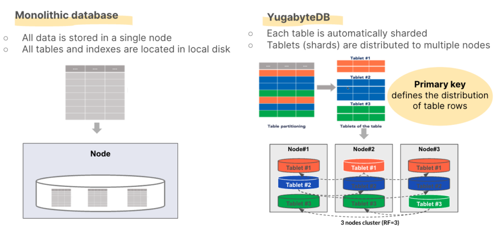
However, traditional databases (like PostgreSQL) and YugabyteDB store data in entirely different ways. This means that as a database engineer, you will still need to do some work to ensure everything works as it should.

Unlike a single-node database that stores all the schema and data on a single disk, YugabyteDB distributes data across multiple nodes, even remote nodes in various zones and regions. Understanding this difference is crucial to ensure a successful migration.

Monolithic database vs YugabyteDB

In this blog post, we will examine how you can migrate data and schema from an existing database to YugabyteDB using YugabyteDB Voyager. We will focus on data modeling for appropriate data distribution and explore two different migration approaches: the Lift path and the Lift & Shift path.

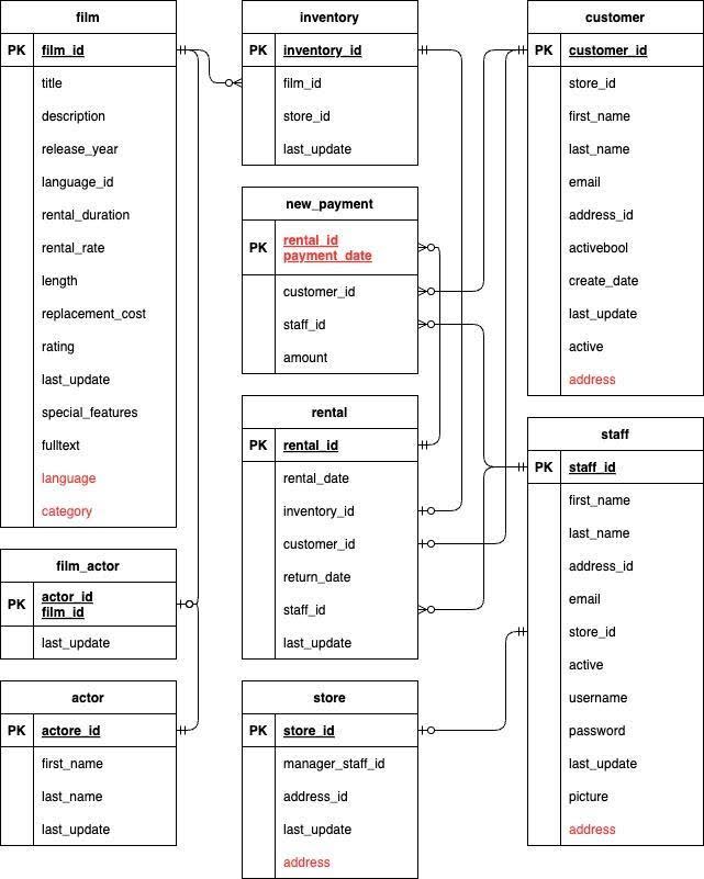
Sample database and scenario

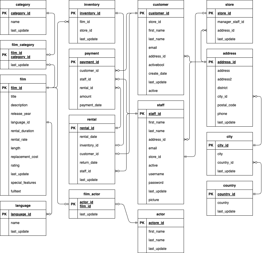
For this example we have used the DVD rental data model, which we picked up from this PostgreSQL tutorial, plus some assumpted use cases (queries) for those tables. If you want to try the migration steps using this data model, download the zip file from the tutorial site and import it to your PostgreSQL database.

Sample database and scenario

table name	rows	growth rate	use cases (query patterns)
actor	200	mid	select a.first_name, a.last_name from actor a join film_actor fa on a.actor_id=fa.actor_id join film f on f.film_id=fa.film_id where f.title=$1 select f.title, f.description, f.release_year from film f join film_actor fa on f.film_id=fa.film_id join actor a on fa.actor_id=a.actor_id where a.last_name=$1
address	603	high	joined with customer, store, staff tables
category	16	low	joined with film table
city	600	low	joined with address table
country	109	low	joined with address table
customer	599	high	SELECT co.country, ci.city, a.address, a.district, a.postal_code, c.first_name, c.last_name from customer c JOIN address a ON c.address_id=a.address_id JOIN city ci ON ci.city_id=a.city_id JOIN country co ON co.country_id=ci.country_id JOIN store s ON s.store_id=c.store_id WHERE s.store_id=$1;
film	1000	mid	SELECT f.title, f.description FROM film f JOIN language l ON f.language_id=l.language_id JOIN film_category fc ON f.film_id=fc.film_id JOIN category c ON fc.category_id=c.category_id WHERE c.name=$1 AND f.release_year > $2 AND f.rating IN ($3,$4) AND l.name=$5
film_actor	5462	mid	joined with film and actor tables
film_category	1000	mid	joined with film table
inventory	4581	high	joined with rental table
language	6	low	joined with film table
payment	14596	high	SELECT r.rental_id, r.rental_date, r.return_date, p.payment_date, p.amount from payment p JOIN rental r ON r.rental_id=p.rental_id WHERE r.rental_id=$1 ORDER BY p.payment_date DESC; INSERT INTO payment (customer_id, staff_id, rental_id, amount,payment_date) VALUES ($1,$2,$3,$4,$5);
rental	16044	high	INSERT INTO rental (inventory_id, customer_id, staff_id, rental_date) VALUES ($1,$2,$3,$4); UPDATE rental return_date=now() WHERE rental_id IN (select rental_id from rental from inventory_id=$1 ORDER BY rental_date DESC LIMIT 1);
staff	2	mid	joined with rental and payment table
store	2	mid	joined with inventory, customer table

Assess the Migration with YugabyteDB Voyager

You can download and install YugabyteDB Voyager for your environment setup here.

Once the sample database is up and running in PostgreSQL, run the following command for the migration assessment. (Note: migration assessment is in the tech preview of Voyager 1.7.0)

yb-voyager assess-migration --export-dir ./export \
        --source-db-type postgresql \
        --source-db-host localhost \
        --source-db-user postgres \
        --source-db-name dvdrental \
        --source-db-schema public

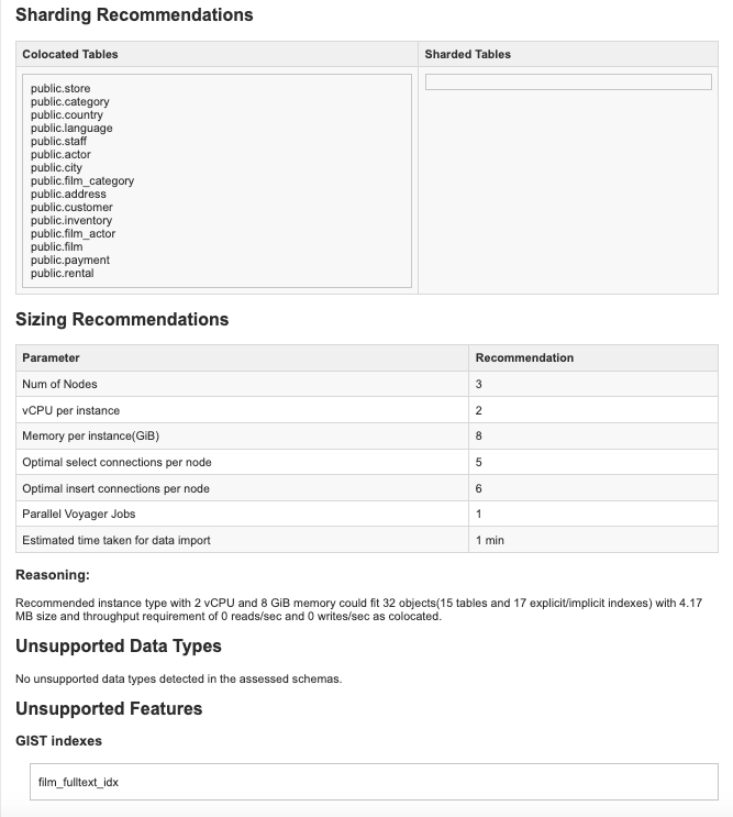
The assessment report will be generated in the /assessment/reports folder under the export directory specified as a command parameter. It contains some recommendations on sharding and cluster sizing, as well as a schema overview and incompatibility.

Sharing Recommendations

Export Schema and Data with YugabyteDB Voyager

YugabyteDB Voyager supports both offline and online migration. Here we will pick the offline path as we don’t have a running application for DVD rental database.

Export schema from PostgreSQL database.

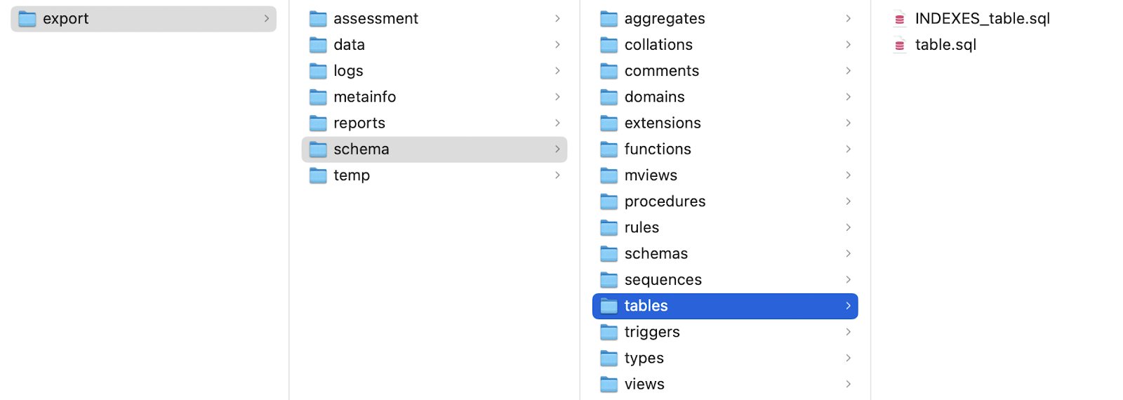
yb-voyager export schema --export-dir ./export \
        --source-db-type postgresql \
        --source-db-host localhost \
        --source-db-user postgres \
        --source-db-name dvdrental \
        --source-db-schema public

The exported schema files are in multiple folders in the export folder.

Then, you can analyze the schema to see if it can be migrated to YugabyteDB.
```
yb-voyager analyze-schema --export-dir ./export --output-format txt
```
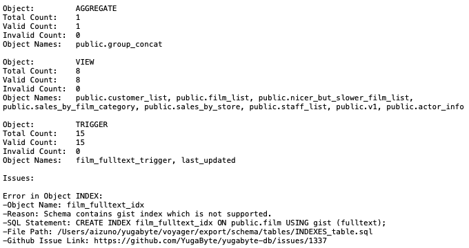
The report is located in the reports folder under the export folder. You will find the issue related to the gist reported at the bottom, because it is not yet supported by YugabyteDB.
You can delete or comment out DDL for film_fulltext_index in INDEX_tables.sql and rerun the analysis report. You will see no issue.

Now you can export data using the command below.

yb-voyager export data --export-dir ./export \
        --source-db-type postgresql \
        --source-db-host localhost \
        --source-db-port 5432 \
        --source-db-user postgres \
        --source-db-name dvdrental \
        --source-db-schema public

You will find the exported data (DML) in the data subfolder.

Lift Path

Users often consider distributed SQL as it provides zero-downtime operation with rolling maintenance or fault tolerance at the zone or region level.

They expect the power of horizontal scalability in the future, but scalability is not always their first requirement.

In these cases, data distribution is less important than the cost of application changes. Users often don’t want to change their application code when they migrate it from their existing data platform to YugabyteDB. For these users, the Lift path is the best way forward.

The DVD rental database doesn’t have big tables with many rows, so we can assume the transaction volume does not exceed the capability of a single node. As the assessment report from YugabyteDB Voyager recommended, colocation is a good way to migrate the DVD rental database with minimum changes.

Import Schema and Data into the Colocation Database

Only the colocation database can hold colocated tables. Once you create a YugabyteDB cluster in your local environment or with YugabyteDB Managed, you can create a colocation database as the migration target database using the YSQL command below.

Create a colocation database in the YugabyteDB cluster.
```
CREATE DATABASE col_dvdrental WITH COLOCATION=true;
```
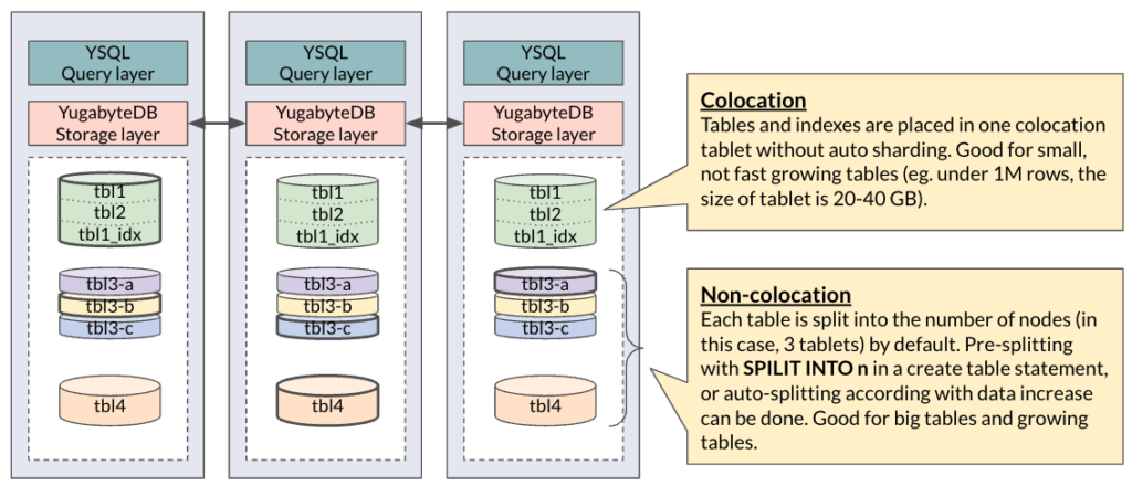
All tables and indexes are colocated by default within the colocation database. Auto sharding is disabled and data is ordered by the primary key. You don’t need to care about data distribution – because data is not distributed in the colocation database.

Import schema into col_dvdrental database.

yb-voyager import schema --export-dir ./export \
        --target-db-host  localhost \
        --target-db-port 5433 \
        --target-db-user yugabyte \
        --target-db-name col_dvdrental

Import data into the col_dvdrental database. Note: unique indexes are also created and populated with this command.

yb-voyager import data --export-dir ./export \
        --target-db-host  localhost \
        --target-db-port 5433 \
        --target-db-user yugabyte \
        --target-db-name col_dvdrental \
        --parallel-jobs 1

Create indexes and populate materialized views with the following command.

yb-voyager import schema --export-dir ./export \
        --target-db-host  localhost \
        --target-db-port 5433 \
        --target-db-user yugabyte \
        --target-db-name col_dvdrental \
        --post-snapshot-import true \
        --refresh-mviews true

After confirming all import commands above are executed without errors, finalize the migration with the end command option.

yb-voyager end migration --export-dir ./export \
        --backup-log-files=true \
        --backup-data-files=true \
        --backup-schema-files=true \
        --save-migration-reports=true \
        --backup-dir ./backup

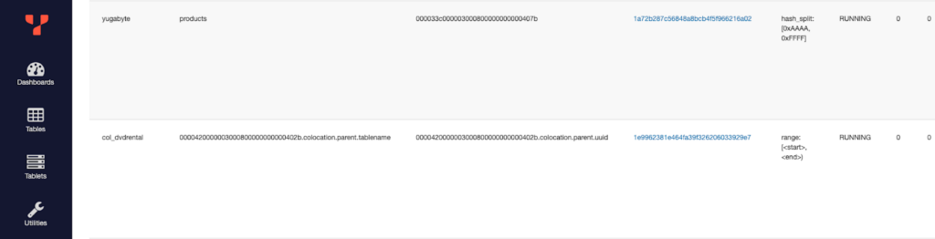
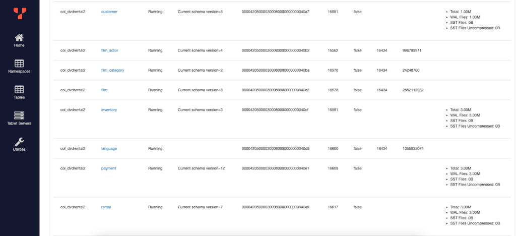
The end command will drop the ybvoyager_metadata schema and three tables that store migration metadata. You can see the list of tables and the number of tablets per node with yugabyted console if you want to check the migration result.

To see the distribution of a specific tablet among the cluster (e.g., the colocation tablet), you can access tserver console and see only one user data tablet for col_database. In the colocation database, all 15 tables are colocated in one tablet, which is replicated to three copies, as RF=3, to form the RAFT group.

Colocation Tablet

Cost-Based Optimizer

In addition to colocation, you can enable YugabyteDB Cost-Based Optimizer to get postgres-like query performance.YugabyteDB 2.21 uses Rule-Based Optimizer by default. We can change the optimizer to cost-based, to utilize the statistics for better query plan selection. If you want to compare a PostgreSQL cost model and YugabyteDB cost model, you can follow the instructions described in this blog post .

\c col_dvdrental
ANALYZE;
SET yb_enable_optimizer_statistics=on;
SET yb_enable_base_scans_cost_model=true;

Query From Colocated Tables

Let’s run queries to migrated tables in YugabyteDB. Since all tables are colocated in the lift migration scenario, queries will run just like a single node postgreSQL.

We use three queries to capture the characteristics of the DVD rental data model.

Search for films: when the customer wants to find films to watch, they specify some conditions to filter the list. (Note: the first run takes longer to plan. I will use the results of the third run of each query execution.)

explain analyze
SELECT f.title, f.description FROM film f
    JOIN language l ON f.language_id=l.language_id
    JOIN film_category fc ON f.film_id=fc.film_id
    JOIN category c ON fc.category_id=c.category_id
WHERE c.name='Action'
    AND f.release_year > 2000
    AND f.rating IN ('G','PG')
    AND l.name='English';
                                                                       QUERY PLAN
----------------------------------------------------------------------------------------------------------------------------------------------------------
 Nested Loop  (cost=13.82..11579.53 rows=4 width=109) (actual time=12.932..15.281 rows=27 loops=1)
   Join Filter: (fc.category_id = c.category_id)
   Rows Removed by Join Filter: 345
   ->  Index Scan using category_pkey on category c  (cost=2.47..375.58 rows=1 width=4) (actual time=3.543..3.546 rows=1 loops=1)
         Remote Filter: ((name)::text = 'Action'::text)
   ->  Merge Join  (cost=11.35..11203.18 rows=62 width=111) (actual time=9.324..11.599 rows=372 loops=1)
         Merge Cond: (fc.film_id = f.film_id)
         ->  Index Scan using film_category_pkey on film_category fc  (cost=4.71..1173.88 rows=1000 width=4) (actual time=1.957..2.292 rows=997 loops=1)
         ->  Materialize  (cost=6.65..10026.02 rows=62 width=113) (actual time=7.351..8.754 rows=372 loops=1)
               ->  Nested Loop  (cost=6.65..10025.87 rows=62 width=113) (actual time=7.309..8.516 rows=372 loops=1)
                     Join Filter: (f.language_id = l.language_id)
                     ->  Index Scan using film_pkey on film f  (cost=4.71..9650.73 rows=372 width=115) (actual time=6.188..7.060 rows=372 loops=1)
                           Filter: (((release_year)::integer > 2000) AND (rating = ANY ('{G,PG}'::mpaa_rating[])))
                           Rows Removed by Filter: 628
                     ->  Materialize  (cost=1.94..369.55 rows=1 width=4) (actual time=0.003..0.003 rows=1 loops=372)
                           ->  Index Scan using language_pkey on language l  (cost=1.94..369.55 rows=1 width=4) (actual time=1.085..1.085 rows=1 loops=1)
                                 Remote Filter: (name = 'English'::bpchar)
 Planning Time: 1.166 ms
 Execution Time: 15.593 ms
 Peak Memory Usage: 502 kB
(20 rows)

Select customer addresses: when the store sends out direct mails to customers, store staff needs to list customer addresses for printing.

explain analyze
SELECT co.country, ci.city, 
  a.address, a.district, a.postal_code,
  c.first_name, c.last_name from customer c
JOIN address a ON c.address_id=a.address_id
JOIN city ci ON ci.city_id=a.city_id
JOIN country co ON co.country_id=ci.country_id
JOIN store s ON s.store_id=c.store_id
WHERE s.store_id=1;
                                                                      QUERY PLAN
--------------------------------------------------------------------------------------------------------------------------------------------------------
 Nested Loop  (cost=2989.50..5878.87 rows=326 width=65) (actual time=14.777..16.835 rows=326 loops=1)
   ->  Seq Scan on store s  (cost=1.34..363.25 rows=1 width=4) (actual time=2.826..2.831 rows=1 loops=1)
         Remote Filter: (store_id = 1)
   ->  Hash Join  (cost=2988.16..5512.35 rows=326 width=67) (actual time=11.936..13.717 rows=326 loops=1)
         Hash Cond: (ci.country_id = co.country_id)
         ->  Hash Join  (cost=2458.34..4978.05 rows=326 width=60) (actual time=9.899..11.411 rows=326 loops=1)
               Hash Cond: (a.city_id = ci.city_id)
               ->  Hash Join  (cost=1123.23..3638.46 rows=326 width=51) (actual time=6.831..8.093 rows=326 loops=1)
                     Hash Cond: (a.address_id = c.address_id)
                     ->  Index Scan using address_pkey on address a  (cost=4.43..2514.14 rows=603 width=40) (actual time=2.985..3.733 rows=603 loops=1)
                     ->  Hash  (cost=1114.72..1114.72 rows=326 width=17) (actual time=3.796..3.796 rows=326 loops=1)
                           Buckets: 1024  Batches: 1  Memory Usage: 25kB
                           ->  Seq Scan on customer c  (cost=4.43..1114.72 rows=326 width=17) (actual time=3.456..3.587 rows=326 loops=1)
                                 Remote Filter: (store_id = 1)
               ->  Hash  (cost=1327.61..1327.61 rows=600 width=15) (actual time=3.038..3.038 rows=600 loops=1)
                     Buckets: 1024  Batches: 1  Memory Usage: 37kB
                     ->  Index Scan using city_pkey on city ci  (cost=4.43..1327.61 rows=600 width=15) (actual time=1.980..2.377 rows=600 loops=1)
         ->  Hash  (cost=528.45..528.45 rows=109 width=13) (actual time=1.980..1.980 rows=109 loops=1)
               Buckets: 1024  Batches: 1  Memory Usage: 14kB
               ->  Index Scan using country_pkey on country co  (cost=3.51..528.45 rows=109 width=13) (actual time=1.819..1.881 rows=109 loops=1)
 Planning Time: 0.915 ms
 Execution Time: 17.148 ms
 Peak Memory Usage: 406 kB
(23 rows)

Update payments: when the customer rents or returns DVDs, their payments are recorded in the database.

explain (analyze, dist)
INSERT INTO payment 
    (customer_id, staff_id, rental_id, amount,payment_date)
VALUES (43,1,123,50.0,now());
                                          QUERY PLAN
------------------------------------------------------------------------------------------------
 Insert on payment  (cost=0.00..0.02 rows=1 width=32) (actual time=0.261..0.261 rows=0 loops=1)
   ->  Result  (cost=0.00..0.02 rows=1 width=32) (actual time=0.010..0.010 rows=1 loops=1)
         Storage Table Write Requests: 1
         Storage Index Write Requests: 3
 Planning Time: 0.072 ms
 Trigger for constraint payment_customer_id_fkey: time=12.189 calls=1
 Trigger for constraint payment_rental_id_fkey: time=3.893 calls=1
 Trigger for constraint payment_staff_id_fkey: time=5.176 calls=1
 Execution Time: 21.733 ms
 Storage Read Requests: 5
 Storage Read Execution Time: 15.825 ms
 Storage Rows Scanned: 6
 Storage Write Requests: 4
 Catalog Read Requests: 0
 Catalog Write Requests: 0
 Storage Flush Requests: 0
 Storage Execution Time: 15.825 ms
 Peak Memory Usage: 149 kB
(18 rows)

Lift & Shift Path

Some users consider migrating to distributed SQL because of its write scalability. However, the best way to distribute data depends on schema, query pattern, data volume, and performance requirements.

YugabyteDB Voyager implements and will make recommendations on sharding and sizing, but users still need to understand and design their data distribution.

Distribute or colocate: Big tables with massive rows are better distributed, but small and slow growing tables are not. Small reference tables should be considered colocation.
Sharding and ordering: If tables are queried by range, the data should be ordered and sharded by its range. The primary key should be specified with ASC or DESC to be range-sharded.
Indexing: Distributed SQL sometimes requires a more aggressive approach to indexing, especially to achieve the expected performance from complex join and aggregation queries.

In a real case, we choose colocation for tables with less than 1 million rows, or smaller than 1 GB, so that the colocation tablet would be 20-40GB at maximum with ~20% compression.

YSQL Query layer

Tablet Size and Data Modeling

Our sample database is relatively small, and no table has millions of rows. As the migration assessment report of YugabyteDB Voyager recommended, we don’t need to distribute the DVD rental database. However, we will distribute some tables and denormalize some parts of the data model to anticipate future data growth.

We will modify our data model based on query patterns, as shown below.

Distribute or colocate
- Distribute: customer, inventory, payment, rental
- Colocate: film, film_actor, actor, store, staff
- Denormalize: language, category, film_category, address, city, country
Sharding and ordering
- customer: customer_id Hash
  - Point query with customer_id is the main usage
  - No range query with customer_id
  - last_name can be queried by range; idx_last_name should be range-sharded
- inventory: inventory_id Hash
  - Point query with inventory_id is the main usage
  - Point query with film_id and store_id; idx_store_id_film_id should be sharded with (film_id Hash, store_id ASC) because film_id is a more selective condition.
- payment: rental_id Hash, payment_date DESC
  - Point query with rental_id or customer_id or staff_id; no query with payment_id
  - rental_id is most selective but not unique; the primary key should be (rental_id Hash, payment_date DESC)
- rental: rental_id Hash
  - Point query with inventory_id filtered by most recent rental_date, and point query with customer_id; no query with rental_id
  - rental_id is the foreign key of payment table, which cannot be deleted
  - idx_unq_rental_rental_date_inventory_id_customer_id may need to be investigated for tuning, but we make this to be range-sharded because the rental table has the index for inventory_id (idx_fk_inventory_id)
    - (rental_date DESC, inventory_id ASC, customer_id ASC)

Sharing Ordering

Schema Modification (Before Data Migration)

We will modify DDLs to reflect the changes to the data model described in the previous section.

You can change schema in the source database, intermediate SQL files, and the target database. Since we assume that our data size is big, minimum data move/rewrite is important to choose the modification method.

So, we modify the schema only to specify colocation or distributed table and index column ordering before the data migration. Denormalization, change of the primary key, and tuning would be done after the data migration.

Open table.sql file under the schema/tables folder in the export folder.

Add WITH (colocation=false) SPLIT INTO n TABLETS to customer, inventory, payment, and rental tables. You can omit the number of splitting tables if it is the same as the number of nodes.

CREATE TABLE public.customer (
    ...omitted...
) WITH (colocation=false) SPLIT INTO 1 TABLETS;

CREATE TABLE public.inventory (
    ...omitted...
) WITH (colocation=false) SPLIT INTO 3 TABLETS;

CREATE TABLE public.payment (
    ...omitted...
) WITH (colocation=false) SPLIT INTO 3 TABLETS;

CREATE TABLE public.rental (
    ...omitted...
) WITH (colocation=false) SPLIT INTO 3 TABLETS;

Open INDEXES_table.sql file under the schema/tables folder in the export folder.

Comment out lines 19 – 28 and 37 – 43 so that the migration process does not create indexes for denormalized and recreated tables.

-- CREATE INDEX idx_fk_address_id ON public.customer USING btree (address_id);
-- CREATE INDEX idx_fk_city_id ON public.address USING btree (city_id);
-- CREATE INDEX idx_fk_country_id ON public.city USING btree (country_id);
-- CREATE INDEX idx_fk_customer_id ON public.payment USING btree (customer_id);
-- CREATE INDEX idx_fk_language_id ON public.film USING btree (language_id);
-- CREATE INDEX idx_fk_rental_id ON public.payment USING btree (rental_id);
-- CREATE INDEX idx_fk_staff_id ON public.payment USING btree (staff_id);

Add the sharding method (Hash or ASC/DESC) and SPLIT INTO n TABLETS to the indexes of non-colocated tables at lines 34, 46 – 52, and 61. You can omit the number of splitting if it is the same as the number of nodes.

CREATE INDEX idx_fk_inventory_id ON public.rental USING btree (inventory_id Hash) SPLIT INTO 3 TABLETS;

CREATE INDEX idx_fk_store_id ON public.customer USING btree (store_id ASC);

CREATE INDEX idx_last_name ON public.customer USING btree (last_name ASC);

CREATE INDEX idx_store_id_film_id ON public.inventory USING btree (film_id Hash, store_id ASC) SPLIT INTO 3 TABLETS;

CREATE UNIQUE INDEX idx_unq_rental_rental_date_inventory_id_customer_id ON public.rental USING btree (rental_date DESC, inventory_id ASC, customer_id ASC);

Import Schema and Data into the Colocation Database

The colocation database can hold both colocated tables and non-colocated tables. In order to lift & shift a database in the desired state, we want to create a colocate database as the target database.

CREATE DATABASE col_dvdrental2 WITH COLOCATION=true;

Then, we can import schema and data from the export directory (e.g. ./export2) with the same yb-voyager command used in the lift path. This time you will find some tables are distributed among the nodes in tserver and master server console.

Colocation Database

Schema Modification (After Data Migration)

In this step we will create enums and integrate small tables into the parent table so that the data model will be denormalized and simplified. The first targets are language, category, and film_category tables whose parent table is film table.

Create an enum for language and add a language column to the film table.

CREATE TYPE lang AS ENUM (
    'English',
    'Italian',
    'Japanese',
    'Mandarin',
    'French',
    'German'
);

ALTER TABLE public.film ADD COLUMN language lang;

UPDATE public.film SET language='English' where language_id=1;
UPDATE public.film SET language='Italian' where language_id=2;
UPDATE public.film SET language='Japanese' where language_id=3;
UPDATE public.film SET language='Mandarin' where language_id=4;
UPDATE public.film SET language='French' where language_id=5;
UPDATE public.film SET language='German' where language_id=6;

In the same way, you can denormalize category and film_category tables.

CREATE TYPE ctgy AS ENUM (
    'Action',
    'Animation',
    'Children',
    'Classics',
    'Comedy',
    'Documentary',
    'Drama',
    'Family',
    'Foreign',
    'Games',
    'Horror',
    'Music',
    'New',
    'Sci-Fi',
    'Sports',
    'Travel'
);

ALTER TABLE public.film ADD COLUMN category ctgy;

UPDATE public.film SET category='Action'
Where film_id IN (
    SELECT film_id from film_category where category_id=1
);
UPDATE public.film SET category='Animation'
Where film_id IN (
    SELECT film_id from film_category where category_id=2
);

...omitted...

UPDATE public.film SET category='Travel'
Where film_id IN (
    SELECT film_id from film_category where category_id=16
);

After validating the data population, you can delete the language_id column in film table, and language, category, and film_category tables.

Next, we will denormalize address, city, and country tables and integrate those data into customer, staff, and store tables as a column with JSONB data type.

ALTER TABLE public.customer ADD COLUMN address jsonb;
ALTER TABLE public.store ADD COLUMN address jsonb;
ALTER TABLE public.staff ADD COLUMN address jsonb;

do
$
declare
    addr_count integer;
    addr_store integer[]=(select array_agg(address_id) from public.store);
    addr_staff integer[]=(select array_agg(address_id) from public.staff);
    addr jsonb;
begin
    SELECT count(*) INTO addr_count FROM address;

    for counter in 1..addr_count loop

      SELECT jsonb_build_object(
        'address_id', a.address_id,
        'address', a.address,
        'address2', a.address2,
        'district', a.district,
        'city_id', a.city_id,
        'city', ci.city,
        'country', co.country,
        'postal_code', a.postal_code,
        'phone', a.phone
      ) INTO addr
      from address a
      join city ci ON ci.city_id=a.city_id
      join country co ON co.country_id=ci.country_id
      where a.address_id=counter;

      IF counter=ANY(addr_store) then
        UPDATE public.store SET address=addr
        where address_id=counter;
      ELSIF counter=ANY(addr_staff) then
        UPDATE public.staff SET address=addr
        where address_id=counter;
      ELSE
        UPDATE public.customer SET address=addr
        where address_id=counter;
      END IF;

    end loop;
end;
$;

After the data validation, you can delete address_id column from customer, staff, and store tables and drop address, city, and country tables.Finally, we will change the primary key of the payment table. However, changes to the primary key constraint will result in rewriting the whole table in YugabyteDB. Instead of altering the existing table, which requires at least two times of rewriting, you can create a new table with a different primary key.

Create new_payment table and insert data from payment table.

CREATE TABLE public.new_payment(
    customer_id smallint NOT NULL,
    staff_id smallint NOT NULL,
    rental_id integer NOT NULL,
    amount numeric(5,2) NOT NULL,
    payment_date timestamp without time zone NOT NULL,
    CONSTRAINT new_payment_pkey 
        PRIMARY KEY (rental_id Hash, payment_date DESC),
    CONSTRAINT new_payment_customer_id_fkey 
        FOREIGN KEY (customer_id) 
        REFERENCES public.customer(customer_id)
        ON UPDATE CASCADE ON DELETE RESTRICT,
    CONSTRAINT new_payment_rental_id_fkey
        FOREIGN KEY (rental_id)
        REFERENCES public.rental(rental_id)
        ON UPDATE CASCADE ON DELETE SET NULL,
    CONSTRAINT new_payment_staff_id_fkey
        FOREIGN KEY (staff_id)
        REFERENCES public.staff(staff_id)
        ON UPDATE CASCADE ON DELETE RESTRICT
) WITH (COLOCATION = false) SPLIT INTO 3 TABLETS;

INSERT INTO public.new_payment
    SELECT customer_id,staff_id,rental_id,amount,payment_date
    FROM public.payment;

We commented out the create statements for indexes on payment table. There were three indexes (customer_id, store_id, rental_id) on payment table, and one of which is covered with the new primary key (rental_id). We will create the rest of them for new_payment table.
```
CREATE INDEX new_idx_fk_customer_id ON public.new_payment USING lsm (customer_id);
CREATE INDEX new_idx_fk_staff_id ON public.new_payment USING lsm (staff_id);
```
After the data validation, you have the option to drop or rename the original table and alter the name of new_payment table to payment table.

Query and Tuning for the New Data Mode

Let’s run queries as we did before and see the difference between two databases.

First, we analyze and gather the statistics of the migrated database to enable the Cost-Based Optimizer.

\c col_dvdrental2
ANALYZE;
SET yb_enable_optimizer_statistics=on;
SET yb_enable_base_scans_cost_model=true;

Search for films: When customers want to find films to watch, they specify some conditions to filter the list.

explain analyze
select title, description from film 
where category='Action' 
    AND release_year > 2000
    AND rating IN ('G','PG')
    AND language='English';
                                                                        QUERY PLAN
------------------------------------------------------------------------------------------------------------------------------------------------------------
 Seq Scan on film  (cost=4.71..9187.99 rows=24 width=109) (actual time=2.649..5.942 rows=27 loops=1)
   Filter: (((release_year)::integer > 2000) AND (rating = ANY ('{G,PG}'::mpaa_rating[])) AND (category = 'Action'::ctgy) AND (language = 'English'::lang))
   Rows Removed by Filter: 973
 Planning Time: 0.280 ms
 Execution Time: 6.082 ms
 Peak Memory Usage: 24 kB
(6 rows)

Since we did not create any indexes for language and category, we would see a seq scan in the query plan. Let’s create a new index to get better performance.

CREATE INDEX idx_language_category ON public.film USING lsm (category, language);

explain analyze
select title, description from film
where category='Action'
    AND release_year > 2000
    AND rating IN ('G','PG')
    AND language='English';
                                                           QUERY PLAN
-----------------------------------------------------------------------------------------------------------------------------------
 Index Scan using idx_language_category on film  (cost=9.41..1242.84 rows=24 width=109) (actual time=5.600..5.651 rows=27 loops=1)
   Index Cond: ((category = 'Action'::ctgy) AND (language = 'English'::lang))
   Filter: (((release_year)::integer > 2000) AND (rating = ANY ('{G,PG}'::mpaa_rating[])))
   Rows Removed by Filter: 37
 Planning Time: 0.492 ms
 Execution Time: 5.747 ms
 Peak Memory Usage: 24 kB
(7 rows)

Select customer addresses: when the store sends out direct mails to customers, store staff need to list customer addresses for printing.

explain analyze
SELECT first_name,last_name,address from customer 
WHERE store_id=1;
                                               QUERY PLAN
-----------------------------------------------------------------------------------------------------------
 Seq Scan on customer  (cost=4.43..6670.12 rows=326 width=240) (actual time=2.414..2.540 rows=326 loops=1)
   Remote Filter: (store_id = 1)
 Planning Time: 0.148 ms
 Execution Time: 2.726 ms
 Peak Memory Usage: 24 kB
(5 rows)

Update payments: when the customer rents or returns DVDs, their payments are recorded in the database.

explain (analyze,dist)
INSERT INTO new_payment
    (customer_id, staff_id, rental_id, amount,payment_date)
VALUES (43,1,123,50.0,now());
                                           QUERY PLAN
------------------------------------------------------------------------------------------------
 Insert on payment  (cost=0.00..0.01 rows=1 width=28) (actual time=0.804..0.804 rows=0 loops=1)
   ->  Result  (cost=0.00..0.01 rows=1 width=28) (actual time=0.010..0.011 rows=1 loops=1)
         Storage Table Write Requests: 1
         Storage Index Write Requests: 2
 Planning Time: 0.139 ms
 Trigger for constraint new_payment_customer_id_fkey: time=10.458 calls=1
 Trigger for constraint new_payment_rental_id_fkey: time=3.444 calls=1
 Trigger for constraint new_payment_staff_id_fkey: time=3.586 calls=1
 Execution Time: 18.437 ms
 Storage Read Requests: 5
 Storage Read Execution Time: 12.422 ms
 Storage Rows Scanned: 6
 Storage Write Requests: 3
 Catalog Read Requests: 0
 Catalog Write Requests: 0
 Storage Flush Requests: 0
 Storage Execution Time: 12.422 ms
 Peak Memory Usage: 145 kB
(18 rows)

Comparing the Query Plans of Two Approaches

We run queries of three use cases for two migration paths. The table below shows the execution summary from each query plan. As you can see, complex queries including four to five tables can be executed in about 20 ms, while simple queries are in 5 ms. Write performance is around 20 ms, but can be improved with efficient index (and primary key) design.

Use case	Lift path (Colocation)	Lift&Shift path (Mixture of non-/colocation with simpler data model)
Search for films	Planning Time: 1.166 ms Execution Time: 15.593 ms Peak Memory Usage: 502 kB	Planning Time: 0.492 ms Execution Time: 5.747 ms Peak Memory Usage: 24 kB
Select customer addresses	Planning Time: 0.915 ms Execution Time: 17.148 ms Peak Memory Usage: 406 kB	Planning Time: 0.148 ms Execution Time: 2.726 ms Peak Memory Usage: 24 kB
Update payments	Storage Table Write Requests: 1 Storage Index Write Requests: 3 Planning Time: 0.072 ms Execution Time: 21.733 ms Peak Memory Usage: 149 kB	Storage Table Write Requests: 1 Storage Index Write Requests: 2 Planning Time: 0.139 ms Execution Time: 18.437 ms Peak Memory Usage: 145 kB

Use case

Lift path (Colocation)

Lift&Shift path (Mixture of non-/colocation with simpler data model)

Search for films

Planning Time: 1.166 ms
Execution Time: 15.593 ms
Peak Memory Usage: 502 kB

Planning Time: 0.492 ms
Execution Time: 5.747 ms
Peak Memory Usage: 24 kB

Select customer addresses

Planning Time: 0.915 ms
Execution Time: 17.148 ms
Peak Memory Usage: 406 kB

Planning Time: 0.148 ms
Execution Time: 2.726 ms
Peak Memory Usage: 24 kB

Update payments

Storage Table Write Requests: 1
Storage Index Write Requests: 3
Planning Time: 0.072 ms
Execution Time: 21.733 ms
Peak Memory Usage: 149 kB

Storage Table Write Requests: 1
Storage Index Write Requests: 2
Planning Time: 0.139 ms
Execution Time: 18.437 ms
Peak Memory Usage: 145 kB

Conclusion

In this blog, we showcased two patterns of migration using the PostgreSQL tutorial model and YugabyteDB Voyager. As demonstrated, the lift path is the easiest way, requiring the least effort and minimal changes. You can then distribute and modify your data model afterward to achieve a more scalable data layer (e.g. lift & shift path).

June 10, 2024