The Benefit of Partial Indexes in Distributed SQL Databases

If a partial index is used, instead of a regular one, on a nullable column—where only a small fraction of the rows have not null values for this column—then the response time for inserts, updates, and deletes can be shortened significantly. As a bonus, the response times for single row selects shorten a little bit too. This post explains what a partial index is, shows how to create one, describes the canonical use case that calls for a partial index, describes some straightforward performance tests, and shows that the results justify the recommendation to use a partial index when you have the appropriate use case.

Introduction

Sometimes, business analysis determines that an entity type has an optional attribute, which remains unset in the typical case, that there is a requirement to identify entity occurrences where the optional attribute is set to some value, and that there is never a requirement to identify occurrences where it is not set. A topical example arises now that some office facilities offer limited bicycle storage in a small basement room and give out a numbered key to the very few employees who take advantage of this. There’s a real need when the janitor hands in a mislaid key, to find out, say, “Who was assigned key #42?” But there’s never a need to identify staff who don’t use the bike storage.

Such an entity type will be implemented as a table that has a nullable column to represent the optional attribute. And the column will need a secondary index to support fast execution of a query that identifies a row by a not null value for this column.

Another case—subtly different from the optional attribute case—arises if you have a table that contains both “billed” and “unbilled” orders, where the “unbilled” orders take up a small fraction of the total table, and yet these are typically the only ones that are the target of select in an OLTP scenario —exactly so that they can be processed and set to “billed”.

A partial index is defined using a restriction so that only some of a table’s rows are indexed. In the present scenario, the restriction will specify, in the first case, that only rows with not null values for this column will be indexed. Or, in the second case, that only “unbilled” rows will be indexed.

This will be beneficial because the partial index will be a lot smaller than a regular index. Most significantly, when rows are inserted or deleted, the maintenance cost of the index will be avoided in the typical case.

“Create index” Syntax

Suppose that we have a table created thus:

create table t(k int primary key, v int);

(I’ll show all SQL statements in this post with a trailing semicolon, as they’d be presented as ysqlsh commands.) Notice that the column t.v is nullable. A regular secondary index is created thus:

create index t_v on t(v);

And a partial secondary index is created thus:

create index t_v on t(v) where v is not null;

The `where` clause restriction can be any single row expression that mentions only columns in the to-be-indexed table. For example, “where v is not null and v != 0”. It’s as simple as that!

Performance tests

I populated table t with 1 Million rows where only ten percent of these had not null values for t.v. Here’s the SQL written in PostgreSQL syntax where the % operator is used to express the modulo function.

insert into t(k, v)
select
a.v,
case a.v % 10
  when 0 then a.v
  else        null
end
from
(select generate_series(1, 1000000) as v) as a;

Test 1: create index

First I created a regular index on t.v, timing the “create index” operation, and ran the timing script. (This script implements Tests #2 through #4.) Then I dropped the index and created a partial index on t.v, timing this operation too, and ran the timing script again.

Test 2: single key select

\timing on
call select_not_null_rows(100000);
\timing off

The procedure select_not_null_rows() simulates OLTP single-row select statements by running a “for loop” implemented thus:

for j in 1..num_rows loop
  select t.k into the_k from t where t.v = the_v;
  the_v := the_v + sparseness_step;
end loop;

Of course, nobody would write a real program like this—especially because, with no unique constraint on t.v, the select statement might return more than one row! But this naïve approach is sufficient for timing purposes. The value of sparseness_step is set to 10, reflecting my choice, expressed via this:

case a.v % 10

in the insert statement, shown above, that I used to populate table t.

The select statement that the procedure repeatedly issues is prepared behind the scenes the first time it is encountered at run time, so that the SQL execution does respect the optimal prepare-execute paradigm.

Test 3: single row insert

\timing on
call insert_rows(100000);
\timing off

The procedure insert_rows() simulates OLTP single-row insert statements by running a “for loop” implemented thus:

for j in 1..num_rows loop
  insert into t(k, v) values(1000000 + j, null);
  commit;
end loop;

Nobody would commit every row in a real program. But it’s this device that simulates single-row OLTP. Here, too, SQL execution respects the optimal prepare-execute paradigm.

Test 4: bulk delete

\timing on
delete from t where k > 1000000;
\timing off

I didn’t use the prepare-execute paradigm here because the time needed for the SQL compilation and planning will be a tiny fraction of the time needed to delete one hundred thousand rows.

Test environments

I recorded the timings in two environments.

• First I used my local MacBook to run a single-node YugabyteDB cluster (Version 2.0.1), with a replication factor (RF) of one. The ysqlsh client was running on the same local machine.
• Then I ran them using a realistic three-node cluster with RF=3, hosted on AWS. I deployed all three nodes in the same “us-west-2” (Oregon) availability zone. The nodes were of type “c5.large”, and each had more than sufficient storage for what my tests required. I ran the ysqlsh client on a separate node in the same availability zone.

Results

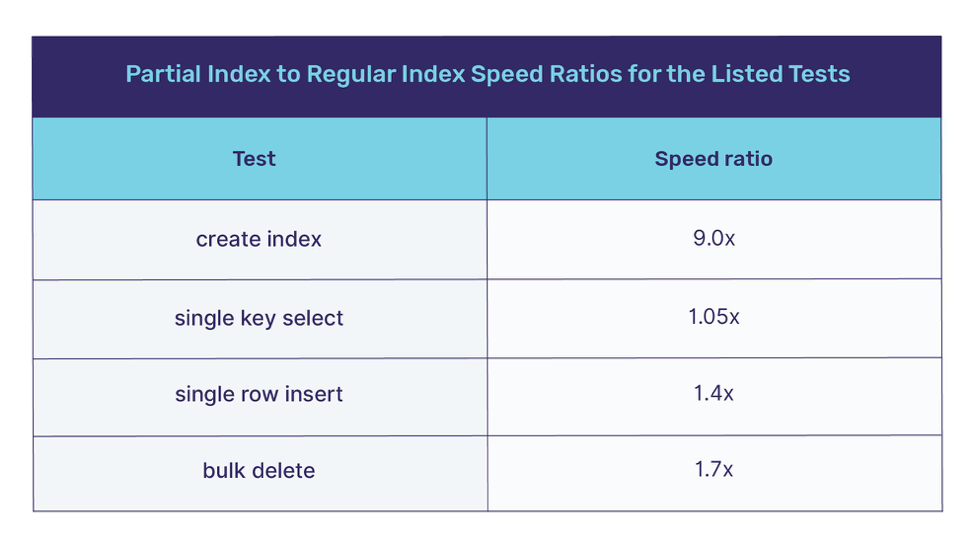
I recorded the elapsed times for the above tests under the two test conditions (regular index and partial index) and in the two test environments (“local” and “cloud”). For every measurement pair, the regular index time was greater than the partial index time. As is to be expected, the absolute values of the times were greater in the “cloud” environment than in the “local” environment. Note that SQL operations on a three-node cluster, with RF=3, using the Raft consensus algorithm and distributed transactions, are expected to be slower than a single node, with RF=1 with no inter-node communication and shorter code paths. There are well-documented benefits to such a resilient and scalable system that may outweigh this cost.

I normalized the results by expressing them as a speed ratio. For example, if a test took 60 seconds using a regular index and 20 seconds using a partial index, then the partial index speed is 3x that of the regular index speed. The speed ratios came out to be the same in the two test environments, within the limits of the accuracy of my measurements.

Of course, your results might be different. A sparser density of not null values in the indexed column will make the speed ratios greater; and a less sparse density will make them smaller.

Conclusion

This post has shown how using a partial index, for an appropriate use case, can reduce the cost of secondary index maintenance and thereby speed up insert, update, and delete operations on the table in question. Reducing the number of secondary index maintenance operations by using partial indexes is especially beneficial in a distributed SQL database such as YugabyteDB. This is because during index maintenance, a transaction that seemingly inserts, updates, or deletes just a single row, automatically becomes a distributed transaction involving the primary row and the secondary index row. Such a distributed transaction can be a multi-shard transaction when the primary row and the secondary index row are present on two different shards on potentially two different nodes of the cluster. As one can imagine, multi-shard shard transactions are inevitably more expensive than single-shard transactions.

What’s Next?

• Compare Yugabyte DB in depth to databases like CockroachDB, Google Cloud Spanner and MongoDB.
• Get started with Yugabyte DB on macOS, Linux, Docker, and Kubernetes.
• Contact us to learn more about licensing, pricing or to schedule a technical overview.