Boosting Performance for Small Distributed SQL Data Sets with Colocated Tables

An Introduction to Colocated Tables

In YugabyteDB v2.1, we released a new feature in beta: colocated tables. And we were excited to announce the general availability of colocated tables, along with many other exciting new features, in YugabyteDB 2.2. In this post, we’ll explain what colocated tables are in a distributed SQL database, why you would need them, and how to get started.

Relational databases often have a large number of tables and indexes. A lot of these tables are closely related and commonly queried together via joins or subqueries. In YugabyteDB, a scale-out distributed SQL database, each table will be split automatically into a number of shards. Sharding is the process of breaking up large tables into smaller chunks called shards that are spread across multiple servers. A shard (also referred to as a tablet) is a horizontal data partition that contains a subset of the total data set, and is responsible for serving a portion of the overall workload. The idea is to distribute data that can’t fit on a single node onto a cluster of database nodes.

So, let’s say you have 1000 tables, each with 1 index. If each table and index is split in 10 tablets, then there are 20000 tablets in the cluster. Each tablet uses its own RocksDB instance to store data. This is done so that the tablets can be uniformly distributed across multiple disks on a node. This example would then result in 20K RocksDB instances, increasing CPU, disk, and network overhead.

Having multiple tablets for small tables that are closely related can be detrimental to performance in a distributed SQL database. This is because complex queries involving joins and subqueries on these tables will result in a large fan-out, requiring lookups across multiple nodes or regions, and incurring network latency. Colocated tables allow you to store (or co-locate) such datasets on a single tablet, called the colocation tablet, thereby eliminating query fan-out and boosting performance. Note that the data in colocated tables is still replicated across multiple nodes, providing high availability, while also making reads much faster.

Starting with YugabyteDB v2.1, you can create a database that is colocated. This will cause all tables in that database to be stored on the same tablet. Large tables or tables with higher write throughput can be opted out of colocation. This will end up creating separate tablets for such tables. You can find more information in the colocated tables documentation.

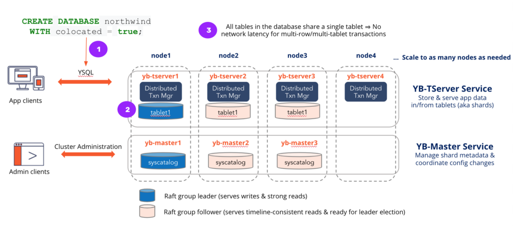
As shown in the above diagram, creating a colocated database will create a single tablet for that database which is replicated across multiple nodes. Data for all tables in that database will be stored on the same tablet. Tables that opt out of colocation will continue to be split into multiple shards.

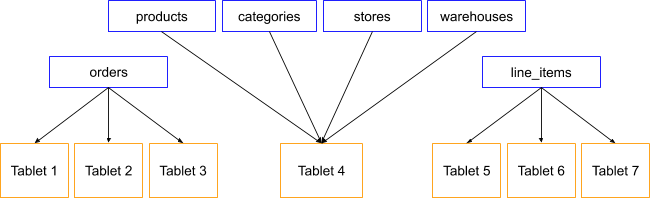
Above is an example of a database using colocated tables. The “products”, “categories”, “stores”, and “warehouses” tables are colocated on a single tablet while the “orders” and “line_items” tables have their own set of tablets.

Use Cases for Colocated Tables

Now that we’ve described what colocated tables are, let’s look at some of the use cases where colocation will be useful:

• Small datasets needing high availability or geo-distribution: An example is a geo-distributed application, such as an identity service, with a small dataset footprint of 500 GB or less. In this case, the identity tables can be colocated onto the same colocation tablet.

• Large datasets that include a few large tables that need to scale out and many small tables: An example here is an IoT application that may contain information from connected devices in a number of tables, but only a few of those tables contain real-time events data. In this case, you can colocate the small tables onto a single shard and the large tables can use their own set of tablets and scale out.

• A large number of databases where each database has a small dataset: An example of an application in this category would be a multi-tenant service. Let’s say you have a thousand databases, one database per customer, but each database size ends up being 500 GB or less. You can colocate the tables within each database onto a single tablet.

While colocation gives you high read performance, it does come with a tradeoff: Since all of your data in the tables now resides on the same tablet, you’re bound by how much data can fit into one tablet. The good news is that this is only applicable until the table(s) are moved out of the co-location tablet, such as when your table data splits into another tablet or you manually move it.

A Real World Example

YugabyteDB itself internally uses colocation to store the system catalog information! The system catalog of YSQL (and PostgreSQL) consists of over 200 tables and relations to maintain metadata information about the database, such as the tables created in the database, columns for each table, indexes, functions, operators, and more. This data is commonly read during query execution and typically involves joins and subqueries across multiple tables. Colocating these tables has helped boost our performance.

As an example, when you run ysql_dump (or pg_dump) to export your database, the query that is fired to get the index definition for the table(s) is shown below:

SELECT 
     t.tableoid, t.oid, t.relname AS indexname,
     inh.inhparent AS parentidx,
     pg_catalog.pg_get_indexdef(i.indexrelid) AS indexdef,
     i.indnkeyatts AS indnkeyatts, i.indnatts AS indnatts,
     i.indkey, i.indisclustered, 
     i.indisreplident, i.indoption,
     t.relpages,
     c.contype, c.conname, c.condeferrable, c.condeferred,
     c.tableoid AS contableoid,
     c.oid AS conoid,
     pg_catalog.pg_get_constraintdef(c.oid, $1) AS condef,
     (SELECT spcname
           FROM pg_catalog.pg_tablespace s
           WHERE s.oid = t.reltablespace) AS tablespace,
     t.reloptions AS indreloptions,
     (SELECT pg_catalog.array_agg(attnum ORDER BY attnum)  
           FROM pg_catalog.pg_attribute  
           WHERE attrelid = i.indexrelid AND attstattarget >= $2)
           AS indstatcols,
     (SELECT pg_catalog.array_agg(attstattarget ORDER BY attnum)  
           FROM pg_catalog.pg_attribute  
           WHERE attrelid = i.indexrelid AND     attstattarget >= $3)
           AS indstatvals
FROM pg_catalog.pg_index i 
     JOIN pg_catalog.pg_class t ON (t.oid = i.indexrelid)
     JOIN pg_catalog.pg_class t2 ON (t2.oid = i.indrelid) 
     LEFT JOIN pg_catalog.pg_constraint c
           ON (i.indrelid = c.conrelid
                AND i.indexrelid = c.conindid
                AND c.contype IN ($4,$5,$6)) 
     LEFT JOIN pg_catalog.pg_inherits inh
           ON (inh.inhrelid = indexrelid)
WHERE i.indrelid = $7::pg_catalog.oid
     AND (i.indisvalid OR t2.relkind = $8)
     AND i.indisready ORDER BY indexname;

As you can see, this is a complex query involving joins across 5 tables, 3 subqueries, and some index lookups!

In a globally-consistent 3-node cluster spanning US-West, US-East, and EU, this query takes ~76 ms. When the above 5 tables are created without colocation, the performance drops by about 50x, and the latency jumps to ~3900 ms!

Colocated Tables in Action

Here’s a demo on how to use colocation and some of the benefits that you can get along the way. For this demo, we have created a globally-consistent YugabyteDB cluster on AWS, with one node in Europe, one in US East, and another in US West. For more information on setting up such geo-distributed clusters, visit YugabyteDB’s multi-DC deployment docs. Ping latencies between the three regions are as follows:

1. EU and US West: 145 ms
2. US East and US West: 60 ms
3. US East and EU: 86 ms

The use of a globally-consistent cluster stretched across 3 data centers far away from each other highlights the full benefits of colocated tables. This is because colocated tables significantly reduce the amount of inter-node communication that happen in the cluster to serve application requests.

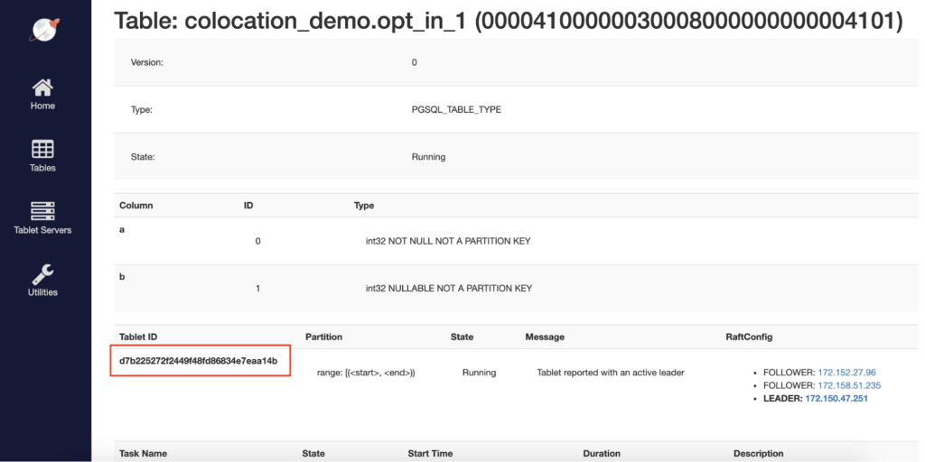
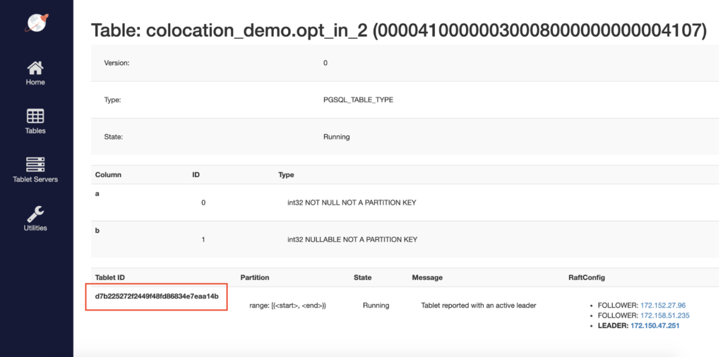
We’ll first create a database called colocation_demo with two tables opt_in_1 and opt_in_2 that are colocated, and two tables opt_out_1 and opt_out_2 that have opted out of colocation. We’ll also create an index on opt_in_1 and opt_out_1.

CREATE DATABASE colocation_demo WITH colocated = true;

CREATE TABLE opt_in_1(a int, b int, PRIMARY KEY(a));
CREATE INDEX ON opt_in_1(b);
CREATE TABLE opt_in_2(a int, b int, PRIMARY KEY(a));

CREATE TABLE opt_out_1(a int, b int, PRIMARY KEY(a)) WITH (colocated = false);
CREATE INDEX ON opt_out_1(b);
CREATE TABLE opt_out_2(a int, b int, PRIMARY KEY(a)) WITH (colocated = false);

The index on table opt_out_1 will be automatically opted out of colocation too since the table opt_out_1 is opted out.

We can verify in the yb-master Admin UI that all opt_in_1 and opt_in_2 tables are on the same tablet.

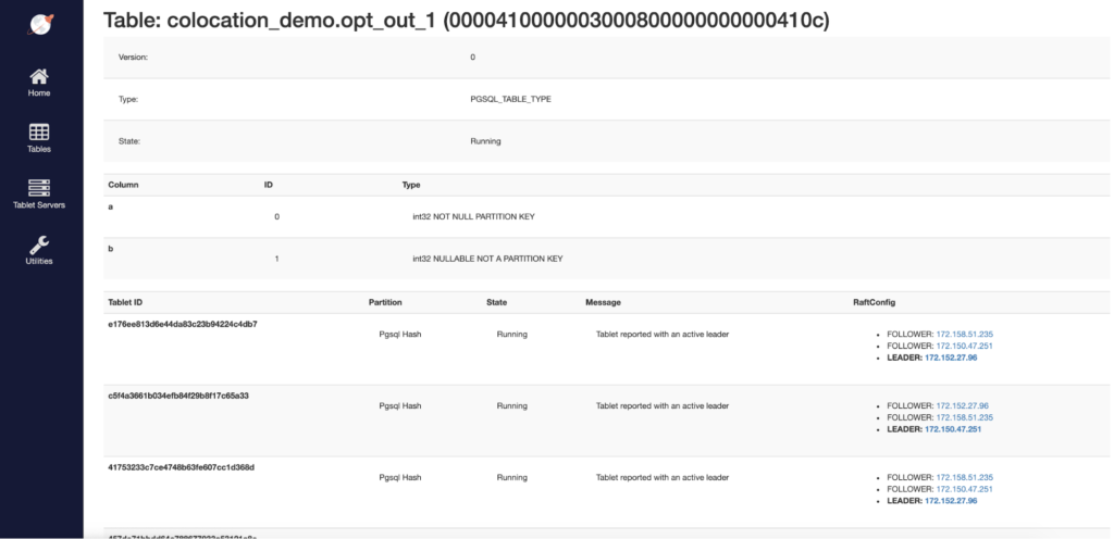
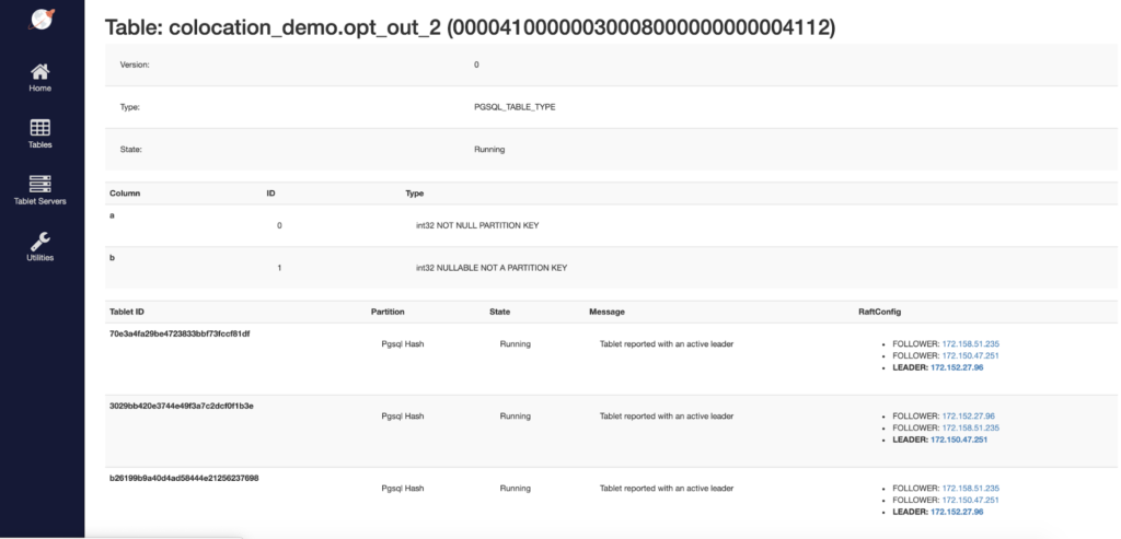
We can also confirm that the opted-out tables, opt_out_1 and opt_out_2, are scaled out across multiple shards (scrolling down in the admin UI will reveal even more shards than are visible in this screenshot).

Next, let’s load the tables with some data and see what the results are when we perform some simple queries.

We’ll load 1M rows in all tables.

INSERT INTO opt_in_1
     SELECT a, a%10 FROM generate_series(1,100000) AS a;
INSERT INTO opt_in_2
     SELECT a, a%10 FROM generate_series(1,100000) AS a;
INSERT INTO opt_out_1
     SELECT a, a%10 FROM generate_series(1,100000) AS a;
INSERT INTO opt_out_1
     SELECT a, a%10 FROM generate_series(1,100000) AS a;

Index lookup

Now, let’s try retrieving some data using the index on opt_in_1 and opt_out_1 tables.

Query:

select * from opt_in_1 where b=6;

colocation_demo=# explain (analyze, costs off) select * from opt_in_1 where b=6;
                            QUERY PLAN                                                           
--------------------------------------------------------------------
Index Scan using opt_in_1_b_idx on opt_in_1  (actual time=11.296..89.092 rows=10000 loops=1)
   Index Cond: (b = 6)
 Planning Time: 0.059 ms
 Execution Time: 89.991 ms
(4 rows)

Time: 90.364 ms

colocation_demo=# explain (analyze, costs off) select * from opt_out_1 where b=6;
                             QUERY PLAN                                                             
----------------------------------------------------------------------
Index Scan using opt_out_1_b_idx on opt_out_1  (actual time=302.582..1628.091 rows=10000 loops=1)
   Index Cond: (b = 6)
 Planning Time: 0.061 ms
 Execution Time: 1629.848 ms
(4 rows)

Time: 1630.278 ms (00:01.630)

As you can see, index lookup for the opted in table was ~18x faster than the opted out table. This is because the index would have retrieved 10K matching rows. Then, for these matching rows, we need to do multiple cross-region reads to get the table rows, resulting in a large fan-out and higher latency.

Update

Let’s now try to update some rows based on a condition on the index.

Query:

update opt_in_1 set b=100 where b=4;

This query will first lookup the index to find all rows matching the condition b=4 (10K such rows), and will then update the table and index with the new value for b for these 10K rows.

colocation_demo=# explain (analyze, costs off) update opt_in_1 set b=100 where b=4;
                            QUERY PLAN                                                              
----------------------------------------------------------------------
Update on opt_in_1  (actual time=7401.463..7401.463 rows=0 loops=1)
   ->  Index Scan using opt_in_1_b_idx on opt_in_1  (actual time=10.986..22.241 rows=10000 loops=1)
         Index Cond: (b = 4)
 Planning Time: 0.055 ms
 Execution Time: 7526.550 ms
(5 rows)

Time: 7587.763 ms (00:07.588)
colocation_demo=# explain (analyze, costs off) update opt_out_1 set b=100 where b=4;
                             QUERY PLAN                                                                 
----------------------------------------------------------------------
Update on opt_out_1  (actual time=15998.822..15998.822 rows=0 loops=1)
   ->  Index Scan using opt_out_1_b_idx on opt_out_1  (actual time=624.430..1800.116 rows=10000 loops=1)
         Index Cond: (b = 4)
 Planning Time: 0.066 ms
 Execution Time: 16236.345 ms
(5 rows)

Time: 16306.560 ms (00:16.307)

In this example, the query on colocated tables is ~2x faster. Notice that the gain here is not as much as the one seen in the other examples. This is because an UPDATE of 10K rows will be uniformly distributed for the opted out table whereas for colocated tables, all 10K updates will go to the same tablet, resulting in a hot shard. So, even though the index read is much faster, the total gain only ends up being 2x.

Let’s now try to update some rows based on a range condition on the primary key.

Query:

update opt_in_1 set b=100 where a<2;

colocation_demo=# explain (analyze, costs off) update opt_in_1 set b=100 where a<2;
                             QUERY PLAN                                                           
----------------------------------------------------------------------
Update on opt_in_1  (actual time=0.775..0.775 rows=0 loops=1)
   ->  Index Scan using opt_in_1_pkey on opt_in_1  (actual time=0.693..0.695 rows=1 loops=1)
         Index Cond: (a < 2)
 Planning Time: 0.585 ms
 Execution Time: 129.615 ms
(5 rows)

Time: 314.916 ms

colocation_demo=# explain (analyze, costs off) update opt_out_1 set b=100 where a<2;
                            QUERY PLAN                                                       
----------------------------------------------------------------------
Update on opt_out_1  (actual time=9331.524..9331.524 rows=0 loops=1)
   ->  Foreign Scan on opt_out_1  (actual time=467.361..9331.441 rows=1 loops=1)
         Filter: (a < 2)
         Rows Removed by Filter: 99999
 Planning Time: 0.049 ms
 Execution Time: 9332.212 ms
(6 rows)

Time: 9395.853 ms (00:09.396)

Here, we see that colocated table performance is ~30x better. The main reason for this is that since colocated tables are stored on a single tablet, they are range sorted by the primary key. This makes range scans a lot more efficient. Opted out tables, on the other hand, are sorted by hash of the primary key. So, this results in a full (and cross-region) scan of the opted-out table.

Joins

colocation_demo=# explain (analyze, costs off) select *
from opt_in_1, opt_in_2
where opt_in_1.a=opt_in_2.a and opt_in_1.b=6;

                             QUERY PLAN                                                              
----------------------------------------------------------------------
Nested Loop  (actual time=11.569..2690.402 rows=10000 loops=1)
   ->  Index Scan using opt_in_1_b_idx on opt_in_1  (actual time=11.184..22.986 rows=10000 loops=1)
         Index Cond: (b = 6)
   ->  Index Scan using opt_in_2_pkey on opt_in_2  (actual time=0.247..0.247 rows=1 loops=10000)
         Index Cond: (a = opt_in_1.a)
 Planning Time: 4.078 ms
 Execution Time: 2693.683 ms
(7 rows)

Time: 2698.550 ms (00:02.699)


colocation_demo=# explain (analyze, costs off) select *
from opt_out_1, opt_out_2
where opt_out_1.a=opt_out_2.a and opt_out_1.b=6;

                             QUERY PLAN                                                                
----------------------------------------------------------------------
Nested Loop  (actual time=312.834..706187.075 rows=10000 loops=1)
   ->  Index Scan using opt_out_1_b_idx on opt_out_1  (actual time=251.379..2157.824 rows=10000 loops=1)
         Index Cond: (b = 6)
   ->  Index Scan using opt_out_2_pkey on opt_out_2  (actual time=70.367..70.367 rows=1 loops=10000)
         Index Cond: (a = opt_out_1.a)
 Planning Time: 4.189 ms
 Execution Time: 706194.641 ms
(7 rows)

Time: 706200.404 ms (11:46.200)

In this example too, colocation helps reduce the query fan-out thus resulting in lower latency of almost 260x.

Summary

Colocated tables (generally available starting with YugabyteDB 2.2) can support a large number of databases and inter-related tables. We hope this post has demonstrated that you can do this very easily with colocation because you’re automatically reducing the number of tablets and reducing the overhead on your YugabyteDB clusters. Colocation is intended for small datasets and can be useful to boost performance while maintaining the automatic scale out architecture across multiple shards for larger tables where needed. We invite you to try out colocated tables and join us in Slack if you have any questions or feedback!

Editor’s note – This post was updated July 2020 with new release information